Fundamentals and Practices of Sensing Technologies
by Dr.
Keiji Taniguchi, Hon. Professor of
Xi’ an
Dr. Masahiro Ueda, Professor of Faculty of Education and Regional Studies
Dr. Ningfeng Zeng, an Engineer of Sysmex Corporation
(A Global Medical
Instrument Corporation),
Dr. Kazuhiko Ishikawa, Assistant Professor
Faculty of Education and
Regional Studies,
[Editor’s Note: This paper is presented as Part III of a series of chapters from the new book “Fundamentals and Practices of Sensing Technologies”; subsequent chapters will be featured in upcoming issues of this Journal.]
1.4 Outlines of GPS
1.4.1 Introduction (1), (21)
The Global Positioning System (GPS) developed by the
US Air Force, provides world-widely a three dimensional position![]() , and velocity information
, and velocity information ![]() for users. The
satellite constellation consists of 24 satellites in
20000(Km) orbits. These satellites are usually broadcasting ranging
codes and navigation data on three frequency bands of L1, L2 and L5 using a
Code Division Multiple Access (CDMA) method. Therefore, the same
frequencies with different ranging codes are used for all satellites. The GPS
system consists of a dual-use system, and is used for the Standard Positioning Service
(SPS) for civil user and the Precise Positioning Service (PPS) for
military one. The L1 and L2 frequency bands are used for the legacy system, and
the L1(1575.92MHz), L2(1227.5MHz), and L5 (1176.45 MHz) frequency bands are
used for the modernized one.
for users. The
satellite constellation consists of 24 satellites in
20000(Km) orbits. These satellites are usually broadcasting ranging
codes and navigation data on three frequency bands of L1, L2 and L5 using a
Code Division Multiple Access (CDMA) method. Therefore, the same
frequencies with different ranging codes are used for all satellites. The GPS
system consists of a dual-use system, and is used for the Standard Positioning Service
(SPS) for civil user and the Precise Positioning Service (PPS) for
military one. The L1 and L2 frequency bands are used for the legacy system, and
the L1(1575.92MHz), L2(1227.5MHz), and L5 (1176.45 MHz) frequency bands are
used for the modernized one.
In this section, the legacy system is described.
1.4.2 GPS System Configurations (1)
Figure 1.42 shows the GPS system configuration. This system consists of three
segments : a space segment, a user segment, and a control segment.

The space segment is consists of 24 satellites with 4 satellites in 6 orbit planes,
and these satellites broadcast the radio wave frequencies of 1575.92(MHz) in L1 band,
and 1227.5(MHz) in L2 band as navigation signals.
The control segment consists of a ground based master control station, and five monitor
stations for tracking the satellites.
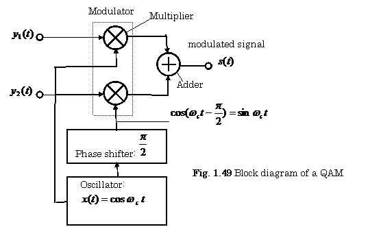
1.4.3 Determination of User Positions (21)
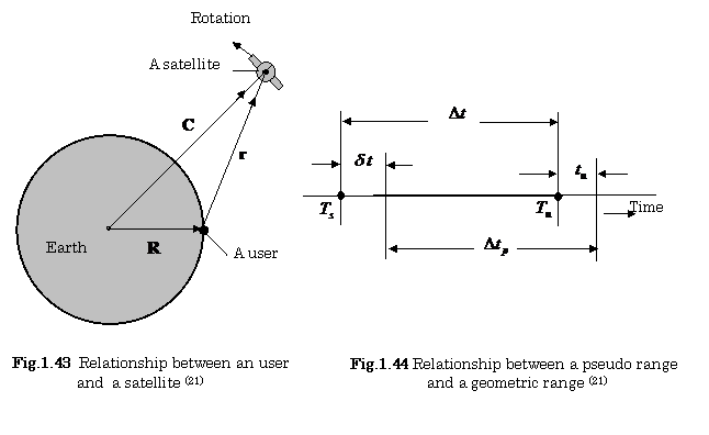
A Relationship Satellite and User
Figure.1.43 shows the relationship between a satellite and a user on the earth.
In this figure, a satellite- to- user vector ![]() is expressed as follows:
is expressed as follows:
![]() (1.14)
(1.14)
The magnitude ![]() of vector
of vector ![]() is also expressed as
follows:
is also expressed as
follows:
![]() (1.15)
(1.15)
where ![]() ,
, ![]() and
and ![]() are the radius of the
earth, a distance between the satellite and the user, and a distance between
the center of the earth and the satellite, respectively.
are the radius of the
earth, a distance between the satellite and the user, and a distance between
the center of the earth and the satellite, respectively.
B. Calculation of Equivalent Time
Figure 1.44 shows the relationship between a pseudo range and a geometric range.
The geometric range ![]() and pseudo range
and pseudo range ![]() are expressed as
follows:
are expressed as
follows:
![]() (1.16)
(1.16)
![]() (1.17)
(1.17)
where we assume that ![]() is negligible small because
an atomic clock(See Fig.1.46) is used as a
main oscillator of all the GPS satellites.
is negligible small because
an atomic clock(See Fig.1.46) is used as a
main oscillator of all the GPS satellites.
In this figure, ![]() is the equivalent time based on a geometric range,
is the equivalent time based on a geometric range, ![]() is the equivalent time based on a pseudo range,
is the equivalent time based on a pseudo range, ![]() is the starting time that the signal left from the
satellite,
is the starting time that the signal left from the
satellite, ![]() is the arrival time
that the signal reached to a receiver of the user,
is the arrival time
that the signal reached to a receiver of the user, ![]() is the off- set time in the clock of the satellite,
is the off- set time in the clock of the satellite,
![]() is the off- set
time in the clock of the user, and
is the off- set
time in the clock of the user, and ![]() is the propagation
speed of radio waves (
is the propagation
speed of radio waves (![]() ).
).
Therefore, Eq. (1.17) can be simplified as follows:
![]() (1.18)
(1.18)
In above equation, ![]() can be measured by a
satellite-generated ranging code information of a received signal.
can be measured by a
satellite-generated ranging code information of a received signal.
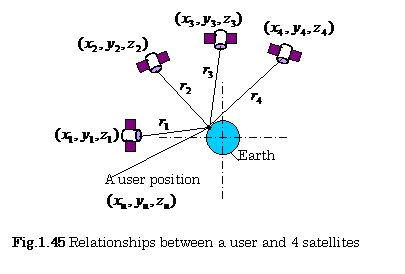
C. Calculation of User Position
Only three unknown user position ![]() would be required if a clock in the user receiver were
synchronized with a clock in the satellite. The clock of a crystal oscillator
in the user receiver is usually employed to determine it’s own position, but
this clock is not so accurate as the atomic clock. Consequently, four unknown
measurements
would be required if a clock in the user receiver were
synchronized with a clock in the satellite. The clock of a crystal oscillator
in the user receiver is usually employed to determine it’s own position, but
this clock is not so accurate as the atomic clock. Consequently, four unknown
measurements ![]() are required (The symbol
are required (The symbol![]() is shown in Fig.1.44). We need at least the ranging codes
information from four satellites by time of arrival (TOA) measurements
as shown in Fig.1.45. The following equation can, then, be obtained from Eq.(1.18):
is shown in Fig.1.44). We need at least the ranging codes
information from four satellites by time of arrival (TOA) measurements
as shown in Fig.1.45. The following equation can, then, be obtained from Eq.(1.18):
![]() ,
, ![]() (1.19)
(1.19)
where ![]() , and
, and ![]() ,
, ![]() express the coordination
of
express the coordination
of ![]() th satellite positions.
th satellite positions.
.
The pseudo range ![]() between the satellite
and the user’s receiver can be computed by measuring the propagation time of
radio waves, which is modulated by a satellite-generated ranging code.
between the satellite
and the user’s receiver can be computed by measuring the propagation time of
radio waves, which is modulated by a satellite-generated ranging code.
The unknown user position ![]() and clock offset of the receiver
and clock offset of the receiver ![]() can be defined as the sum
of the approximate components
can be defined as the sum
of the approximate components![]() ,
,![]() ,
,![]() ,
, ![]() , and the incremental components
, and the incremental components![]() ,
,![]() ,
,![]() ,
,![]() , as follows:
, as follows:
![]() ,
, ![]() ,
, ![]() ,
, ![]() (1.20)
(1.20)
We also define the pseudo ranges as follows:
![]()
![]() ,
, ![]() (1.21).
(1.21).
The pseudo range ![]() can be obtained as a
linear approximation as follows by means of the Tailor expansion series:
can be obtained as a
linear approximation as follows by means of the Tailor expansion series:
![]()
![]()
[![]()
![]()
![]()
![]()
![]()
![]()
![]()
![]()
![]()
![]() (1.22).
(1.22).
where
![]()
 ,
, ![]()

![]()
 ,
, ![]() ,
,
![]() , .
, .
![]()
![]()
(1.23)
Substituting Eq.(1.21) and Eq.(1.23) into Eq.(1.22), the pseudo range ![]() can be
can be
expressed as follows:
![]()


Rearranging the above equation,
![]()


 ,
, ![]() (1.24)
(1.24)
For simplicity, we put as follows:
![]() ,
,
 ,
,  ,
, 
then Eq. (1.24) can be described as follows:
![]()
![]() (1.25).
(1.25).
Furthermore, a matrix expression of Eq.(1.25) are as follows:
![]()

 (1.26)

![]() (1.27)
(1.27)
D. Calculation of User Velocity
(a)
The user velocities can be obtained by calculating the differentiation of Eq.(1.25 ) as follows:
![]()
![]() (1.28).
(1.28).
where, we put as follows :
![]() ,
, ![]() ,
, ![]() ,
, ![]() ,
, ![]()
Eq.(1.25 ) is, then, rewritten as follows:
![]()
![]() (1.29)
(1.29)
where ![]() can be obtained
from the ranging code.
can be obtained
from the ranging code.
However, practically, this method is not so accurate for noise problems.
(b) Carrier Doppler Phase Shift Method
A carrier Doppler phase shift ![]() arises by the relative
motion between the satellite and the user, and is expressed as follows:
arises by the relative
motion between the satellite and the user, and is expressed as follows:
![]() (1.30)
(1.30)
In the above equation,
![]() ,
,![]() ,
,![]() ,
,![]() ,
,
![]() (1.31)
(1.31)
where ![]() is the transmitting
frequency,
is the transmitting
frequency, ![]() is the receiving
frequency,
is the receiving
frequency, ![]() is the satellite-to- user relative velocity,
is the satellite-to- user relative velocity, ![]() is the velocity of the
satellite(
is the velocity of the
satellite(![]() ),
), ![]() is the unit vector
pointing along the line of sight from the user to the satellite(
is the unit vector
pointing along the line of sight from the user to the satellite(![]() ) ,
) , ![]() is the propagation speed of radio waves,
is the propagation speed of radio waves,![]() is the measured estimate of the receiving frequency, and
is the measured estimate of the receiving frequency, and ![]() is the drift rate of
the user clock. The following equation is, then, obtained from Eqs.(1.30) and
(1.31),.
is the drift rate of
the user clock. The following equation is, then, obtained from Eqs.(1.30) and
(1.31),.
![]()
![]()

,![]() (1.32)
(1.32)
The user velocity ![]() can, thus be obtained by
processing carrier phase measurements due to the Doppler frequency shift.
can, thus be obtained by
processing carrier phase measurements due to the Doppler frequency shift.
1.4.4 Configurations of GPS Transmitter and Receiver (21)
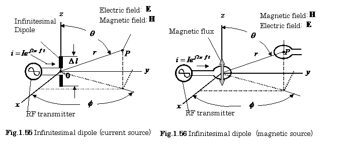
A. Configurations of GPS Transmitter
Figure 1.46 shows a block diagram
of the GPS transmitter. The satellite frequency ![]() , which is generated by means of the highly accurate free
running atomic clock, expresses the main oscillator. Two elements, BPSK and
QPSK, express a binary phase shift keying modulator and a quardrature phase
shift keying modulator (See comment 1.2).
, which is generated by means of the highly accurate free
running atomic clock, expresses the main oscillator. Two elements, BPSK and
QPSK, express a binary phase shift keying modulator and a quardrature phase
shift keying modulator (See comment 1.2).
A symbol ![]() expresses an exclusive
OR operation (modulo two addition), and its operation is defined as follows:
expresses an exclusive
OR operation (modulo two addition), and its operation is defined as follows:
![]() .
.
Prior to the QPSK modulation, the 50 bps navigation message data is combined with both the coarse/acquisition code (C/A code) and the precision code (P(Y) code).
Figures 1.48 (a),(b),(c) and (d) show the basic configuration of the BPSK Modulator, a carrier waveform, a data signal waveform, and a modulated waveform, respectively.
Transmitting signal L1, and L2 of the GPS transmitter are ![]() , and
, and ![]() , respectively.
, respectively.
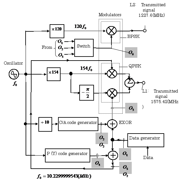
Fig.1.46 Simplified block diagram of the GPS
Transmitter
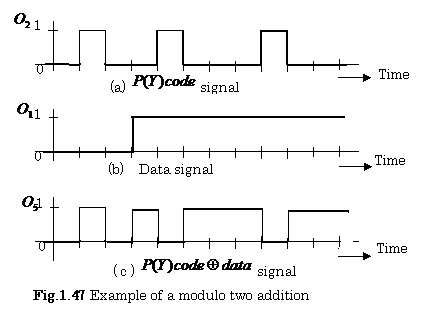
【Example 1.15】Figures1.47 (a)
and1.47 (b) show an example of signal waveforms of a ![]() code(
code(![]() shown in Fig.1.46) , and data(
shown in Fig.1.46) , and data(![]() shown in Fig.1.46), respectively.
shown in Fig.1.46), respectively.
Find the waveform of ![]() .
.
【Solution】: The waveform
of ![]() shown in Fig.1.46 is expressed as Fig.1.47( c ).
shown in Fig.1.46 is expressed as Fig.1.47( c ).
【Comment 1.2】Modulations:
The following modulators are used in the GPS system.
(1) Binary Phase Shift Keying (BPSK) Modulator
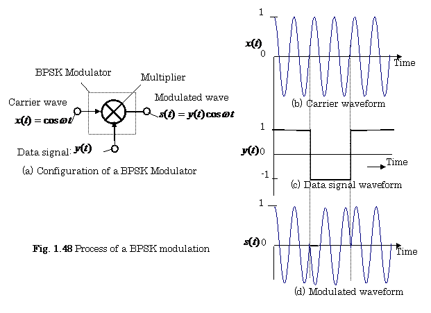 Figure
1.48 shows the configuration of a BPSK modulator and its signal waveforms.
Figure
1.48 shows the configuration of a BPSK modulator and its signal waveforms.
(2) Quadrature Phase Shift Keying(QPSK)Modulator
Figure 1.49 shows the configuration of a QPSK modulator. This modulator
consists of two BPSK modulators, and has the following two data signal inputs: ![]() and
and![]() . The output signal of this modulator is expressed as:
. The output signal of this modulator is expressed as: ![]() .
.
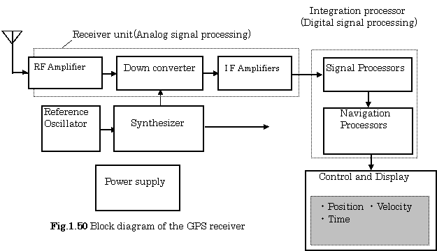
B. Configurations of GPS Receiver
Figure 1.50 shows a block diagram of the GPS receiver. The GPS receiver consists of five principal components: an antenna, a receiver, an integration processor, a control and display units, and a power supply.
The user receiver determines at least pseudo ranges, and also determines pseudo range rates by the Doppler measurements of its own- clock frequency.
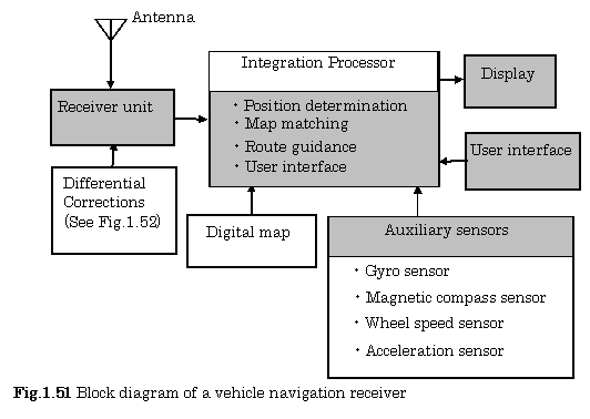
Figure 1.51 shows a block diagram of a vehicle navigation receiver.
The vehicle navigation receiver has auxiliary sensors for an integrated processor as shown in Fig.1.51, and then can calculate the optimized user position.
The digital road map is also used for looking-up the nearest street address.
1.4.5 Differential GPS Systems (21)
The Differential GPS (DGPS) is used for improving the positioning and timing performance of GPS user by means of one or more reference stations whose positions are precisely known. Figure 1.52 shows a differential GPS system configuration.
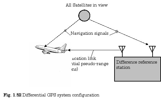
These systems can eliminate some of errors containing commonly in the user and the reference station. These errors are satellite clock errors, satellite position errors, tropospheric errors, and ionospheric errors.
1.4.6 Other navigation systems (21)
There exist other navigation systems except the GPS:
A. European Union Gallileo Satellite System
The Gallileo Satellite System (GSS) is developing by the European Union (EU). This system consists of 30 satellites in 23222 (Km) orbits. These satellites are usually broadcasting ranging codes and navigation data on L5-E5 (1164-1214MHz), E6 (1260-1300MHz), and E2-L1-E1 (1559-1591MHz) bands, and are fully compatible with the GPS system.
B. Russian Global Navigation Satellite System
The Russian Global Navigation Satellite System (GLONASS) is consists of 24 satellites in 19100(Km) orbits. These satellites are usually broadcasting same ranging code and navigation data in different frequencies on two frequency bands: 1246-1257 (MHz), and 1602-1616 (MHz), using a frequency division multiple access (FDMA) method.
C. Chinese Bei Dou Navigation System
This is the Chinese multistage satellite navigation program designed to Chinese military and civil users.
D. Japanese QZSS Program
This program is to intend the navigation services to address shortfalls in GPS satellite visibility in urban canyons and mountainous terrain.
1.5 Outlines of RFID Tags
1.5.1 Introduction (22)
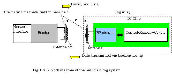
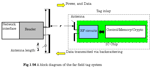
A RFID (Radio Frequency IDetification) system consists of readers (interrogators)
and tags(transponders). A reader communicates with a tag by means of a wireless system and collects information attached in a tag.
There are three types of tags from their operating principles: a passive tag, a semi-passive tag, and an active tag.
1.5.2 Coupling of RFID Tags ( 22)
In the passive tags, there are coupling techniques of two different types:
a near field tag, and a far field tag.
1.5.3 Types of Passive Tags (22)
A. Near Field Tag
Figure 1.53 shows a block diagram of the near field tag system. The frequencies commonly used in this system are 128(KHz), and 13.56(MHz). A disadvantage of this system is that a large antenna coil is required.
The distance ![]() between the reader and
the tags is expressed as follows:
between the reader and
the tags is expressed as follows:
![]() (1.33)
(1.33)
where ![]() is the wavelength of
radio waves (See 1.5.4 B).
is the wavelength of
radio waves (See 1.5.4 B).
B. Far Field Tag
Figure 1.54 shows a block diagram of the far field tag system. The operation frequencies used in this system are 860-960(MHz), or 2.45(GHz) in the UHF band.
The antenna of this
reader (interrogator) is usually designed to the length of ![]() (
(![]() is the wavelength of radio waves).
is the wavelength of radio waves).
The distance ![]() between the reader and
the tags is expressed as follows:
between the reader and
the tags is expressed as follows:
![]() (1.34)
(1.34)
where ![]() is the wavelength of
radio waves (See 1.5.4B).
is the wavelength of
radio waves (See 1.5.4B).
1.5.4 Near and Far Fields of radio waves (23 ),(24), (25)
For designing smaller sizes of tags, some knowledge of antenna pattern is the most important key points. So we will show here these outlines.
A. Electric and Magnetic Fields Intensities
(a) Electric Source Case
An infinitesimal electric dipole antenna (![]() ,
, ![]() is the wavelength of
radio waves) is shown in Fig.1.55. Practically, this antenna can be constructed
by a capacitor-plate in order to maintain the current uniformly on the antenna.
is the wavelength of
radio waves) is shown in Fig.1.55. Practically, this antenna can be constructed
by a capacitor-plate in order to maintain the current uniformly on the antenna.
In Fig.1.55, the ![]() field components,
field components, ![]() ,
, ![]() , and
, and ![]() , and the
, and the ![]() field components,
field components,![]() ,
, ![]() , and
, and ![]() radiated from this antenna,
are expressed as follows:
radiated from this antenna,
are expressed as follows:

![]()
![]()
![]()
![]()
![]() ,
, ![]() ,
, ![]()
![]()
![]()
where ![]() (
(![]() ) is the length of this antenna,
) is the length of this antenna, ![]() is the radial distance
is the radial distance ![]() in the propagation of
radio waves,
in the propagation of
radio waves, ![]() is the intrinsic
impedance of free space,
is the intrinsic
impedance of free space, ![]() is the antenna current, symbol
is the antenna current, symbol ![]() means the definition,
means the definition, ![]() , and
, and ![]() .
.
Furthermore, the ![]() field components,
field components,![]() and
and ![]() express the
intensities of the induction electric field, and static electric field,
respectively.
express the
intensities of the induction electric field, and static electric field,
respectively.
The ![]() field components,
field components,![]() ,
,![]() and
and![]() express the intensities of the radiation electric field, the
induction electric field and static electric field, respectively.
express the intensities of the radiation electric field, the
induction electric field and static electric field, respectively.
The ![]() field components,
field components,![]() and
and ![]() express the
intensities of the radiation magnetic field and the induction magnetic field,
respectively.
express the
intensities of the radiation magnetic field and the induction magnetic field,
respectively.
(b) Magnetic Source Case
Figure 1.56 shows an
infinitesimal magnetic dipole antenna. The ![]() field
field
components,![]() ,
, ![]() , and
, and ![]() radiated from this antenna,
are also expressed as follows:
radiated from this antenna,
are also expressed as follows:

![]()
![]()
![]()
![]()
![]() ,
, ![]() ,
, ![]() ,
,
![]()
![]()
where ![]() is the surface area of
the antenna,
is the surface area of
the antenna, ![]() is the radial distance
is the radial distance ![]() in the propagation of
radio waves,
in the propagation of
radio waves, ![]() is the intrinsic
impedance of free space,
is the intrinsic
impedance of free space, ![]() is the antenna current,
is the antenna current, ![]() ,and
,and ![]() . Furthermore, the
. Furthermore, the ![]() field components,
field components,![]() and
and ![]() express the intensities of the induction magnetic field, and
static magnetic field, respectively.
express the intensities of the induction magnetic field, and
static magnetic field, respectively.
The ![]() field components,
field components,![]() ,
,![]() and
and![]() express the intensities of the radiation magnetic field, the
induction magnetic field and static magnetic field, respectively.
express the intensities of the radiation magnetic field, the
induction magnetic field and static magnetic field, respectively.
The ![]() field components,
field components,![]() and
and ![]() express the intensities
of the radiation electric field and the induction electric field, respectively.
express the intensities
of the radiation electric field and the induction electric field, respectively.
【Example 1. 16】
In Fig.1.56, find the angle ![]() for which the coupling
between the two loop
for which the coupling
between the two loop
antennas vanishes.
【Solution】
From this figure, and Eq. (1.36), we get the following equations:
![]() (1),
(1), ![]() (2),
(2), ![]() (3).
(3).
From these equations, ![]()
![]()
B. Boundary between Near Field and Far Field
InFigs.1.53 and 1.54, when the angle between the transponder antenna and the tag antenna equals to the ninety degree, we get the following equations:
![]() ,
, ![]() ,
,![]() ,
, ![]() ,
,
From these equations, the distance where the induction field equals to the radiation field, is expressed as follows:
![]()
![]() (1.37)
(1.37)
C. Numerical Examples of Boundary between Near Field and Far Field
Table1.2 shows several numerical examples of the boundary between the near field
and the far field intensities calculated by using Eq.(1.37).
![]()
|
Frequency |
Wave
length |
|
|
128(KHz) |
234 |
37.26 |
|
13.56(MHz) |
22.12 |
3.52 |
|
860MHz) |
0.35 |
0.056 |
|
960(MHz), |
0.31 |
0.05 |
|
2.45(GHz) |
0.12 |
0.019 |
1.5.5 Far Field Tags (25 ) , (26), (27)
A. Examples of UHF Tags
Figure 1.57 shows several different types of UHF tags. These tags have the different types of antenna patterns. |
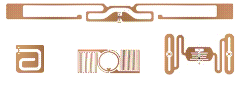
Fig.1.57 Different types of UHF tags(These
figures are reprinted from Ref.(26))
|
Fig.1.57 Different types of UHF tags(These figures are reprinted from Ref.(26))
|
B. Approved Frequency ranges
Table 1. 3 shows the approved frequency ranges where the printers (transponders) are certified(See www.paxar.com).
![]()
|
Countries |
Frequency ranges (MHz) |
|
|
918.5 – 925.5 |
|
|
902 – 928 |
|
EU and EFTA |
869.85 |
|
|
920.5 – 924.5 |
|
|
952 – 955 |
|
|
952 – 954 |
|
|
910 – 914 |
|
|
902 – 928 |
|
|
922 – 927 |
|
|
902 – 928 |
1.5.6 Application Examples of Tags (22) ,(27)
Applications of tags are as follows: supply chain, access control, transport payment, E-pass ports, automotive security, livestock ID, automated libraries, health care,
detecting and locating buried unexploded ordnance (25) , etc,.
【References】
(1)D. Christiansen : Electronics Engineers’ Handbook, 4th Edition, pp.13.1-13.50
IEEE Press (1997)
(2) K. Taniguchi, H. Ozaki: A New Detecting Circuit for Microcell Counters, Electronics and Communications in Japan,Vol.53-C,No.6, pp.386-392(1970)
(3) K. Taniguchi, H. Ozaki: Automatic Microcell Analyzer, Electronics and
Communications in
(4)K.H.Schoenbach, R.Nuccitelli, S.J.Beebe: ZAP, IEEE Spectrum,pp.20-24 (August, 2006)
(5)K. Fujimoto:Princioles of Measurement in Hematology Analyzers manufactured by Sysmex Corporation,pp43-60,Sysmex Journal,Vol.22,No1,(Spring, 1999)
(6)Overview of Automated Hematology analyzer XE-2100TM,Product Development
Division, Sysmex Corporation. pp76-84,Sysmex Journal,Vol.22,No1,(Spring, 1999)
(7)H. Ozaki, K.Taniguchi : Sensors and Signal Processing(2nd Edition),p.34, Kyoritsu Pub. Co. Ltd. (1988), (In Japanese)
(8)K. Taniguchi, H. wakamatsu : Medical Electronics and Biomedical Information, pp.140-141,Kyoritsu Pub. Co. Ltd. (1996), (In Japanese)
(9)Y. Horiike, Y.Miyahara: Bio-chips and Bio-sensors, pp.83-84, Kyoritsu Pub. Co. Ltd. (2006) , (In Japanese)
(10)R. C. Dorf : Electrical Engineering Hand Book, pp.1158-1159,CRC Press (1993)
(11) B.P.Lathi: Modern Digital and Analog Communication Systems -third edition,pp.81-98,Oxford University Press (1998)
(12) A.V. Oppenheim and R. W. Schafer: Discrete-Time Signal Processing, pp.114-115, Prentice Hall (1989)
(13) J.A.Cook,D.McNamara,K.V.Prasad:Control, Computing and Communications:
Technologies for the Twenty-First Century Model T, Proceedings of the IEEE,
Vol.95, No.2, pp.334-355 (2007)
(14) J.Rosen, B. Hannaford : DOC at a DISTANCE, IEEE Spectrum,pp.28-33 (Oct.,2006)
(15) O.Brand: Microsensor Integration Into Systems-on-Chip, Proceedings of the
IEEE , Vol.94, No.6, pp.1160-1176 (2006)
(16) Datasheet, ADXL-203, Analog Devices,
(17)Overview of Automated Hematology analyzer SF-3000TM,Product Development
Division, Sysmex Corporation, Sysmex Journal,Vol.18, pp.11-22(1995)
(18)N.Tatumi,I.Tsuda,T.Takubo,T.Katagami,T.Fukuda and H.Kubota: Evaluation of the automated Hematology Analyzer SF-3000TM, Sysmex Journal,Vol.19, NO.1,
pp.76-83 (Spring1996)
(19)M. Kondo : Radio Wave Information Engineering, pp.75-80,Kyoritsu Pub. Co. Ltd.(1999)
(20) R.Cravotta: Making vehicles safer by making them smarter, EDN 6, pp.49-57 (2006)
(21) E.D.Kaplan, C.J.Hegarty : Understanding GPS : Principles and Applications - 2nd Edition, Artech House (2006)
(22) V. Chawla and D. S. Ha : An Overview of Passive RFID,IEEE Applications and Practice, Vol.45,No.9,(Sept. 2007)
(23) Kazimierz Siwiak: Radiowave Propagation and Antennas for Personal
Communications,2nd Edition, pp.7-24, Artech House (1998)
(24) K. Taniguchi : Antennas and Radio Wave Propagation.pp.76-82,Kyoritsu Pub. Co. Ltd.(2006) ,(In Japanese)
(25) G. Marrocco :The Art of UHF RFID Antenna Design: Impedance Matching and
Size Reduction Techniques, IEEE Antennas & Propagation Magazine,Vol.50,
No1,pp.66-79(Feb.2008)
(26) www.paxar.com (Bar Code and RFID Smart Labels & Tags)
(27)K. A. Shubert, R.J. Davis, T.J. Barnum, and B.D. Balaban: RFID Tags to Aid Detection of Buried Unexploded Ordnance, IEEE Antennas & Propagation Magazine,Vol.50,No5,pp.13-24(Oct..2008)
(28)K. Taniguchi, M. Ueda, K. Ishikawa : Practical Sensing Technologies, Kyoritsu Pub. Co. Ltd.(2008) ,(In Japanese)
Problems and Solutions: |
1.1 Find the inverse Fourier transform ![]() of
of ![]() .
.
【Solution】:
![]()
Let![]() , then
, then ![]() , and
, and ![]() . As a result,
. As a result,
![]()
![]()
![]()
1.2 An
actual analog to digital conversion can not be
executed instantaneously, For this reason, an actual high precision
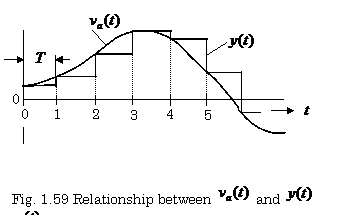
analog to digital (A/D) converter includes a sample and hold (S/H) circuit as
shown in Fig. 1.58. In this figure, the
relationship between ![]() and
and ![]() is shown in Fig. 1.59.
is shown in Fig. 1.59.
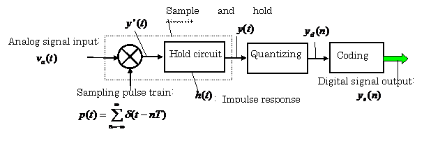
Fig. 1.58 Configuration of an A/D converter including a
S/H circuit
![]()
In these two figures, determine ![]() and
and ![]() .
.
【Solution】:
(1) ![]() , for
, for ![]() ,
, ![]() , for otherwise.
, for otherwise.
(2) ![]()
where ![]()
![]() , *denotes the operation of convolution.
, *denotes the operation of convolution.
1.3 Derive Eq.(1.8).
【Solution】:
(i) If transmitting power ![]() with omni-directional were uniformly radiated in all
direction of a free space, then the power density
with omni-directional were uniformly radiated in all
direction of a free space, then the power density![]() at a distance
at a distance![]() from the antenna would be expressed as follows:
from the antenna would be expressed as follows:
![]() (1)
(1)
(ii) The power is actually radiated from a beam
antenna with gain ![]() . The power density at the center of beam is therefore
expressed as follows:
. The power density at the center of beam is therefore
expressed as follows:
![]() (2)
(2)
(iii) The object with the radar cross section ![]() reflects some of
the power toward the transmitting antenna, since the object operate as a
reflector. The reflecting power
reflects some of
the power toward the transmitting antenna, since the object operate as a
reflector. The reflecting power![]() is then expressed as follows:
is then expressed as follows:
![]() (3)
(3)
(iv) A power density at the location of the transmitting antenna is expressed as follows:
![]() (4)
(4)
(v) The receiving power is expressed as follows:
![]() (5)
(5)
where ![]() is the effective area of the antenna.
is the effective area of the antenna.
(vi) The relationship between![]() and
and ![]() of the antenna is
expressed as follows:
of the antenna is
expressed as follows:
![]() (6)
(6)
where![]() is the wavelength of the transmitting signal and
is the wavelength of the transmitting signal and ![]() is the factor which expresses
the efficiency of the antenna.
is the factor which expresses
the efficiency of the antenna.
(vii) Using the results described above, the receiving power ![]() is expressed as
follows:
is expressed as
follows:
![]() (7)
(7)
1.4 Find the Fourier transform of ![]() :
:
【Solution】:
(1) The inverse Fourier transform of ![]() .
.
![]()
![]()
![]()
Therefore
![]()
![]() 2
2![]()
![]() , and
, and ![]()
![]() 2
2![]()
![]()
(2)Using the Euler’s formula, ![]() .
.
(3)From the result described above, we obtain
![]()
![]()
![]() .
.
As
described above, the spectrum of ![]() consists of two
impulse components.
consists of two
impulse components.
1.5 Find the Fourier transform ![]() of
of ![]() given by:
given by:
![]() ,
, ![]() , for
, for ![]() ,
, ![]() , for
, for ![]() .
.
【Solution】:
![]()


 . Therefore
 ![]()
![]()
![]() .
.
1.6 Derive Eq.(1.35).
【Solution】:
(A) Cartesian Coordinate System:
The vector potential A using the Cartesian coordinate system, is expressed as follows:
![]() (1)
(1)
where ![]() ,
,![]() and
and![]() are the unit vectors
aligned in the
are the unit vectors
aligned in the![]() ,
,![]() and
and ![]() axes, and
axes, and
![]() ,
, ![]() and
and ![]() are the components of
are the components of ![]() aligned in the
aligned in the![]() ,
,![]() and
and![]() axes, respectively.
axes, respectively.
In the case of Fig.1.55, the vector potential is expressed
as: ![]()
where![]() is the current flowing the length
is the current flowing the length ![]() of the ideal
infinitesimal dipole,
of the ideal
infinitesimal dipole, ![]() is the permeability,
is the permeability, ![]() is the radial distance
from the origin of the coordinate system, respectively. The wave number
is the radial distance
from the origin of the coordinate system, respectively. The wave number ![]() is given as:
is given as: ![]() .
.
(B) Spherical Coordinate System:
The vector potential A using the spherical coordinate system, is expressed as follows:
![]() (2)
(2)
where ![]() ,
,![]() and
and![]() are the unit vectors aligned in the
are the unit vectors aligned in the![]() ,
,![]() and
and![]() axes, and
axes, and ![]() ,
, ![]() and
and ![]() are the components of
are the components of ![]() aligned in the
aligned in the![]() ,
,![]() and
and ![]() axes,, respectively.
axes,, respectively.
The relationships between the Cartesian coordinate system and the spherical coordinate system are given as follows:
![]()
![]() (3)
(3)
![]()
(C) Vector Product:
In the spherical coordinate system, the vector product ∇×A![]() is expressed as follows:
is expressed as follows:
(4)
(D) Calculation of Magnetic Fields:
The relationship between the magnetic field![]() and the vector potential
and the vector potential ![]()
is expressed as follows:
(6) (5)
![]() ,
, ![]() ,
,
From the above equations, we can obtain the following equation:
From the above equation, the ![]() field components,
field components, ![]() ,
,![]() and
and![]() are expressed as follows:
are expressed as follows:
(1)![]()
![]() ,
, ![]() (7)
(7)
(2)![]()
![]() ,
, ![]() (8)
(8)
(9)
(3)
![]()
![]() ,
, ![]()
where ![]() ,
, ![]() ,
, ![]() .
.
(G) Calculation of Electric Fields:
The relationship between the electric field![]() and the vector potential
and the vector potential ![]() is
expressed as follows:
is
expressed as follows:
(10) (11)
![]()
,
![]() ,
,
From the above equations, we can obtain the following relations:
![]()
 (12)
(12)
,![]() ,
,![]()
From the above equations, the ![]() field components,
field components, ![]() ,
, ![]() , and
, and ![]() are expressed as
follows:
are expressed as
follows:
(14) (13)
![]()
(15)
![]()
where ![]() ,
, ![]() .
.
(H) Components of Electric Fields:
From Eq. (14), the three electric field components are expressed as follows:.
![]() (1)
Static electric field :
(1)
Static electric field : ![]()
(2) Induction
electric field : ![]() ( 16 )
( 16 )
(3) Radiation electric field
:![]()
1.7 Derive Eq.(1.36).
【Solution】:
(A) Transforming Current Source into Magnetic Source:
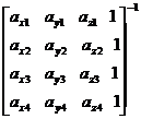
Table 1 shows the relationship between the current source and the magnetic source.
There are the duality between them.
Table 1 Transforming current source into magnetic
source
|
Current source |
|
|
|
|
|
|
|
|
|
|
|
|
|
|
|
|
|
|
|
(B) Component of Magnetic Fields:
(1) By transforming Eq.(1.35 ),we get the following relations:
![]() ,
,![]() ,
,![]() ,
,
where ![]() ,
, ![]() ,
,![]() .
.
(2) By transforming Eq.(1.35 ),we get the following relations:
![]() ,
,![]() ,
,![]()
(C) Component of Electric Fields:
By transforming Eq.(1.35 ),we get the following relations:
![]() ,
,![]() ,
,![]() ,
,
where
![]() ,
, ![]()
![]()
![]()
[ BWW Society Home Page ]
© 2009 The Bibliotheque: World Wide Society