I. Introduction

 

A phenomenon of dynamical chaos or simply chaos became one of the intriguing and remarkable achievements made in science of the 20-th century. It refers to the irregular, unpredictable, and apparently random behavior of deterministic dynamical systems. At the first glance a chaotic behavior in dynamical systems contradicts the universal laws of motion. According to Newton's equations of motion the position and velocity of a system at the certain moment of time is uniquely determined by its position and velocity at the initial instant of time. Its means the future state of the system is fully predictable if its initial conditions are known.

 

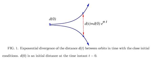
At the end of the 19-th century a French mathematician and physicist Henri Poincaré first noted that a motion of planetary bodies may become unpredictable. In a modern terminology he predicted a chaotic behavior of dynamical systems. He realized that the problem lay not with the universal laws of motion, but with the specification of the initial conditions, "… it may happen that small differences in the initial conditions produce very great ones in the final phenomena. A small error [change] in the former will produce an enormous error [change] in the latter. Prediction becomes impossible …"

 

Later a number of distinguished mathematicians, Emile Borel, Andrei N. Kolmogorov and followers proved that for a vast majority of dynamical systems any small error in initial conditions will be fast growing, and in general exponentially, that the prediction of results will be practically impossible (see Figure 1). These dynamical systems called as chaotic systems exhibit very sensitive dependence on initial conditions.

 

 

         During the second half of the 20-th century many mathematicians and physicists made enormous contributions for understanding and description of this phenomenon in different areas of natural and engineering sciences, even economical sciences [1,2]. A dynamical chaos occurs in wide-range problems of physics, astronomy, chemistry, biology, and ecology. For instance, a particle motion in accelerators, magnetic field lines in magnetically confinement fusion devices, motion of planetary bodies in a Solar system, etc.

 

 In this short paper I would like to describe a simple example, which shows the onset of chaotic motion in so-called Hamiltonian systems. This example also demonstrates some new features of chaotic motion that has been recently found (see Ref. [3] and references therein). For many fundamental models of physical systems whenever dissipation is negligible Newton's equations of motion can be formulated as a set of ordinary differential equations determined only by one master function. This function and the corresponding equations of motion are called Hamiltonian after 19-th century Scotish mathematician R. Hamilton who first introduced them. Below I study the onset of chaotic motion and some its properties in a simple model of Hamiltonian system.

 

II. Particle in a field of two waves

 

Consider a one-dimensional motion of a charged particle in a field of two monochromatic electromagnetic waves propagating along the axis x. The motion of particle is determined by the Newton's equation

 

 where m and e are a mass and an electric charge of a particle, respectively, and E(x,t) is a strength of electromagnetic waves

 

 

 The first wave with the amplitude E₀ propagates with a velocity W₀ along the axis x, while the second wave with the amplitude E₁ is running with the velocity W₁. Suppose that the amplitude of the first wave, E₀  is much larger than the amplitude of the second wave, E₁, i.e. E₀ >> E₁. The parameter c in the equation (2) is a phase difference between waves.

 

To study the motion of particle it is convenient to change a coordinate system x to the new one q= x - W₀ t which moves with the first wave with the velocity, W₀. In the new coordinate system the equations of motion (1) can be reduced to

 

 

where w₀ = (eE₀/m)^1/2 is a frequency of oscillations a physical meaning of which will be cleared below, the quantity W = W₁ - W₀  is a relative velocity of the second wave with respect to the first wave. The parameter e = E₁ /E₀  characterizes a relative amplitude of the second wave.

 

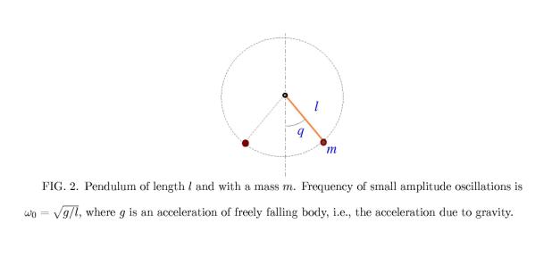
The equation (3) describes also the motion of a pendulum whose a suspension point is oscillating with the frequency W and the amplitude e (see Fig. 2). Then the frequency w₀ coincides with a frequency of small amplitude oscillations of the pendulum.

 

 

Consider first the case of the fixed suspension point when e = 0. The full energy of pendulum is then conserved

 

 

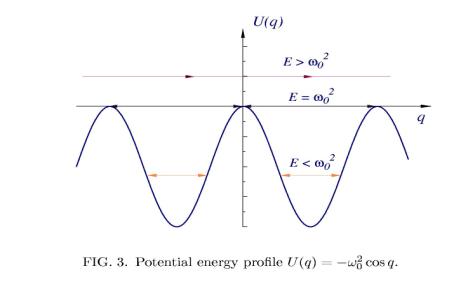
where U(q) is a potential energy shown in Figure 3. There are two kind of motion of the pendulum. When the energy E is less than the maximum of the potential U_max = w₀², i.e., E < w₀² the pendulum oscillates about the lowest point q=0. If  E > w₀² the pendulum rotates around the suspension point. The first case corresponds to the motion of particle trapped in a potential field of the first wave.

 

 

It is convenient to describe a motion on the (q, p)- plane, where p= dq/dt is a momentum. The (q, p)- plane is known as a phase space. An each point on this plane uniquely determines a state of system. The variables (q, p) satisfy to the following system of equations

 

 

For a given initial condition (q₀, p₀) at t = 0 the system of equations (1) has a unique solution (q(t), p(t)). The latter can be displayed by a curve on the (q, p)- plane. The mentioned above two possible types of motion of the pendulum are shown in Figure 4. Arrows indicate directions of motion. There are also so called fixed points where the system is motionless, i.e., the coordinate q and momentum p are fixed: . These points lie on the q- axis with the coordinates (q_n = pn, p=0), (n= 0, ±1,  ±2, . . .). There are two kinds of the fixed points. The points with even numbers (n=2s, (s= 0, ±1,  ±2, . . .) are so-called elliptic fixed points where the potential function U(q) reaches its minimum value U_min(q_2s) = -w₀² . These points are also called O- points since trajectories around them form closed elliptic curves (see Figure 4).

 

 

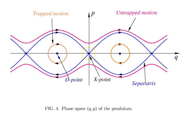
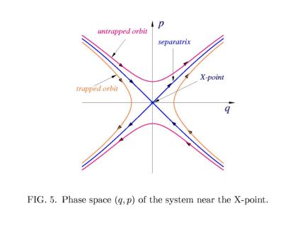
The second kind of the fixed points with odd numbers (n=2s+1, (s= 0, ±1,  ±2, . . .) are called hyperbolic fixed points or X-points. At these points U(q) reaches its maximum value U_min(q_2s+1) = w₀² , and two orbits cross each other transversely. The orbits around the X-point are described by hyperbolic curves. It is seen from the expanded view of the rectangular are of the phase-space area near the X- point marked by the yellow in Figure 4 is shown in Figure 5.

 

As was mentioned above for E < w₀² the pendulum oscillates about the lowest level q = 0, and this regime describes the motion of the particle trapped by the main wave (the orange curves in Figure 4). The pendulum is rotating if E > w₀². It corresponds to particles, which are not trapped by the first wave (magenta curves in Figure 4). The magenta curve above the q- axis (p >0) describes the motion of the un-trapped particle along the positive direction of q, i.e., (), and below the q- axis (p <0) - along the negative direction of q, i.e., (). These two kinds of curves are separated by the phase space curves (the blue curves in Figure 4) crossing each other at the X- points. These curves called as a separatrix correspond to the motion of particle with the energy E equal to the maximum of a potential energy, i.e., E = U_max = w₀² .

 

Consider a motion of particle near the X- point more in a detail (see Figure 5). A particle slows down along both; the trapped and non-trapped orbits when it approaches an area close to the X-point and spend relatively long time in this area. Moreover, if the particle moves along the separatrix it approach the X- point asymptotically, i.e., it will reach this point for infinite time. Let d(t) be a distance from the particle position along the separatrix to the X- point. Then this distance changes with time t as

 

 

where d(t₀) is a distance at the initial time instant t₀. Here a negative sign (-) corresponds to the case if a particle approaches the X- point, and a positive sign (+) describes the case when a particle moves outward the X- point (d(t₀) ¹ 0). A parameter g is determined only system's behavior near the X- point. For the pendulum it is equal to g = w₀. A separatrix is very sensitive to any small external time-dependent perturbations. The latter destroy the separatrix leading to an irregular motion of particle. In the next Section we study this phenomenon.

 

III. Chaotic motion

 

Consider the effect of the second wave with the amplitude E₁ on particle motion in the field of the first wave. As was mentioned above the problem is equivalent to the pendulum whose suspension point oscillates, and it is described by equations (3) with the non-zero perturbation parameter e ¹ 0. This problem is known also a periodically--driven non-linear oscillator.

 

Suppose that the amplitude of perturbation is small, i.e., e <<1. The perturbation disturbs the orbits of the unperturbed pendulum. The disturbance depends on how the orbits are close to the separatrix. The trapped and non-trapped orbits located sufficiently far from the separatrix are only slightly deformed. But orbits, which are close to the separatrix, are affected drastically by the perturbation. A typical behavior of orbits located close to and far from the separatrix is shown in Figure 6. Orbits close to the O-point are only slightly deformed: the distance between the perturbed and the unperturbed orbits with the same initial conditions does not grow (orange curve in Figure 6).

 

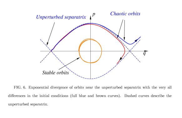
The orbits near the separatrix become very sensitive to the slight change of initial conditions. The distance between two orbits located near the unperturbed separatrix with very close initial coordinates exponentially grows. A typical example of this is shown in Figure 6. Although, each orbit is uniquely determined by it's initial coordinates, even very small difference in initial conditions leads to the dramatic change in a final state of the orbit. Therefore, behavior of the systems near the separatrix becomes unpredictable. Such a phenomenon in dynamical systems is called chaos (or deterministic chaos).

 

A. Poincaré sections

 

Poincaré introduced a powerful tool to study dynamical systems. This tool is based on displaying the coordinates of the orbit (q(t), p(t)) on the phase plane (q, p) taken at periodic time instants t_k = k T  , (k= 0, 1, 2, …) with a period T equal to the period of perturbation 2p/W. The set of points (q_k, p_k) = (q(t_k), p(t_k)) is known a Poincaré section. The relation between two consecutive points (q_k, p_k) and (q_k+1, p_k+1) or the projection of (q_k, p_k)  to (q_k+1, p_k+1):

 

 

               

is called a Poincaré map (more precisely a stroboscopic map).

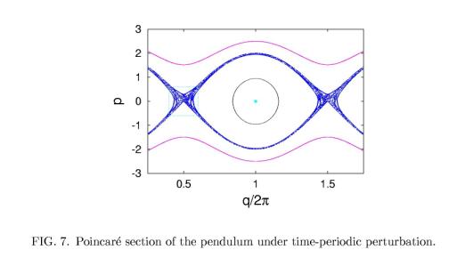
       The Poincaré map is a convenient tool to visualize a behavior of dynamical systems, especially, in a chaotic case. Poincaré section of the periodically driven pendulum described by Eq. (3) is displayed in Figure 7.

 

 

 

 

B.  Stochastic Layer

 

If the orbit is a regular (non-chaotic) the set of points (q_k, p_k) form a closed curve on the phase space (q, p). An example of such orbits is plotted in Fig. 7 by pink and black curves. If the orbit is chaotic the points are scattered on the (q, p) - plane filling the certain region of the phase space. This region is called a stochastic (or chaotic) layer. It is shown in Fig. 7 by blue dots formed near the unperturbed separatrix. The width of the stochastic layer is maximal near the X-points. The stochastic layer is not uniformly filled with the scattered points. 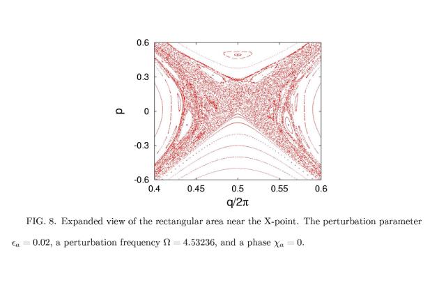There are small regions inside the stochastic layer and its boundary region where orbits have regular (non-chaotic) behavior. These regions called Kolmogorov--Arnold-Moser (or KAM) stability islands (after the mathematicians who proved a theorem on existence such a stability of motion) are clearly seen in Fig. 8 where the expanded view of the rectangle region near the X-point plotted Fig. 7 is shown.

 

 

 

The motion in the stochastic layer is not completely chaotic. There exist intervals of time during of which a motion can be trapped at the border regions of KAM--stability islands. In such time intervals a particle may move around islands almost regular. Duration of the trapping time depends on the structure of each island. However, these trapping events happen occasionally and randomly. One cannot exactly predict a trapping time or its duration, but one can estimate a probability of trapping time durations or in general, a statistical description of motion in the stochastic layer is needed. At the beginning of chaos theory it is expected that a motion in the stochastic layer can be described as a random walk process (similar to Brownian motion) with the Gaussian statistics. Later when computational capabilities were developed, it has been found that in typical chaotic dynamical systems the Gaussian random process cannot always describe irregular motion. It turns out that due to stickiness of motion to the KAM--stability islands the statistics of chaotic motion deviates from the Gaussian one and depends on the structure of the stochastic layer.

 

Below, we will show that the statistics of chaotic motion in a stochastic layer significantly depends on the its topological structure, and its mainly determined by the structure of the stochastic layer near the X-points since particles spend relatively large intervals of time at these areas of a phase space.

 

IV. Rescaling invariance of motion near X-points

 

The width of the stochastic layer is increased with the perturbation parameter e. The structure of the stochastic layer, i.e., the mutual positions of the KAM stability islands, also changes with e. However, the change of the structure is not arbitrary. It has been found that the topological structure of the stochastic layer near the X-points is a periodical function of the logarithm of the perturbation parameter e. In this section we consider this non-trivial property of motion in a stochastic layer, which has been recently established (see Ref. [3] and references therein).

 

We will compare the structures of the stochastic layer for the two sets of perturbation parameter e and its phase c. Let (e_a, c_a) be the first set and (e_b, c_b) be the second set. For these parameters corresponding structures of the stochastic layer are different. However, when these parameter are related according to the following formula:

 

 

the phase--space topologies of the stochastic layer near the X-point corresponding for these two sets of parameters are conserved. The rescaling parameter l in (7) is determined only the parameter g describing the behavior of unperturbed system near the X-point (see Section II) and the frequency of perturbation, W: l= exp(2pg/W). Poincaré sections of the stochastic layer near the X-points plotted Figs. 9 a and b for the perturbation parameters (e_a = 0.02, c_a = 0) and for (e_b = le_a = 0.08, c_b =c_a +p), respectively, clearly show the similarity of the structures. The rescaling parameter l is equal to 4.

 

 

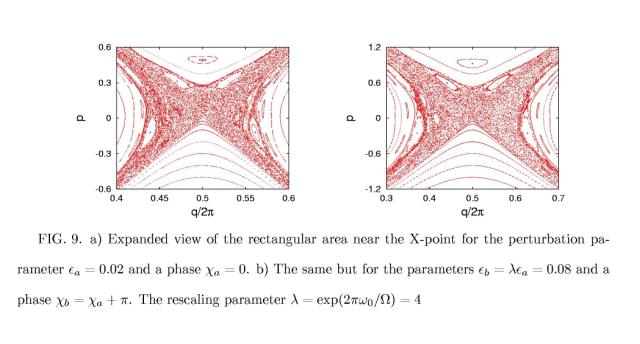
Moreover the phase--space coordinates (x,y) measured with respect to the X-point coordinates, (q_s, p_s), i.e., x= q - q_s, y = p  - p_s, are rescaled according to relation:

 

 

 In Fig. 9 a, b the coordinates x, y are rescaled by factor l^1/2=2.

 

Therefore the structure of the stochastic layer near X-points is a periodic function of the logarithm of the perturbation parameter, log e, and with the period log l= gT, where T is the period time-periodic perturbation subjected to system.

 

 

V. Statistics of chaotic motion in a stochastic layer

 

Since a particle motion in a stochastic layer becomes unpredictable, it does not have a sense to follow each individual orbit. A statistical description of particle motion in a stochastic layer becomes more appropriate.

 

To be more specific we consider statistical properties of chaotic particle motion along the q- axis. Suppose, that at the initial time instant t = 0 a large number, N  >> 1, of particles are located in the stochastic layer near the X-point (q= p, p=0). The initial coordinates of particles are different but close to each other. Each particle will move along the q- axis randomly changing its direction during time evolution (t >0). One of the main statistical characteristics of random motion is a mean square spatial displacement, defined as

 

 

where the angular bracket  <(…)> means a statistical averaging over all particles:

 

 

The quantity s²(t) grows with time t: s²(t)= 2D t^g, where g and D are constants.

 

If the chaotic motion of particle in the stochastic layer could be described as a random walk along the q- axis then the particle transport would be a normal diffusion (Gaussian) process. For this process the exponent g = 1 and the constant D is called a diffusion coefficient. For typical chaotic dynamical systems the exponent g no equal to unity, i.e., g ¹ 1. The case g > 1is called enhanced (or super-diffusive) transport, while the case g < 1is known as a sub-diffusive transport.

 

For our model of particle transport in a stochastic layer the exponent g > 1. It is determined by the structure of the stochastic layer, mainly near the X-points where a particle slows down and spends relatively large time intervals. As was shown above the structure of a stochastic layer near the X-points periodically changes with log e. If the conjecture that similar structures of the stochastic layer give rise to similar transport properties (for instance, the exponents  g), then one can expect that the statistical characteristics of transport are periodic (or quasi-periodic) functions of  log e with the period  log l.

 

A numerical simulation really shows such a log e - periodicity of transport characteristics, which is shown in Fig. 10 for the dependence of the exponent g. 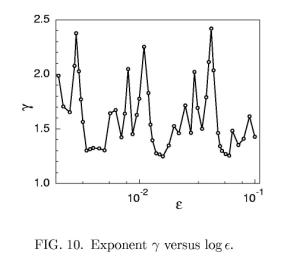 The period of oscillation of g is determined by the rescaling parameter l and equal to log l. It has been also found that the mean square displacement moment s²(t) is also a quasi-periodic function of  log e.

 

This property shows that the chaotic transport rate along a stochastic layer is not a monotonically growing function of the perturbation parameter e, as it was originally believed. It demonstrates that the structure of a stochastic layer near the X-point plays a crucial role in transport processes.

 

 

Conclusions

 

In this paper I have presented the simple example of a chaotic system and demonstrated the "non-chaotic" property of its structure. This property shows that chaotic motion in dynamical systems is not entirely irregular but it has a certain regular statistical properties.

 

At the present time a chaotic behavior in dynamical systems has been found in many branches of physical and engineering sciences, as well as in socio -economical sciences. It plays an important role in understanding of complex, irregular behavior of a wide variety of natural and social phenomena. For readers interested more about a phenomenon of chaos one can recommend a review article [1] and a book [2].

 

 

 References:

 

1.      R.V. Jensen, Chaos, in "Encyclopedia of Physical Sciences and Technology", (Academic Press Inc., 1992) v. 3.

2.    R.C. Hilborn, Chaos and Nonlinear dynamics. An Introduction for Scientist and Engineers, 2-nd Edition (Oxford University Press: New York, 2000).

3.    S.S. Abdullaev (2000) "Structure of motion near the saddle points and chaotic transport in Hamiltonian systems",  Physical Review E, 2000, v. 62, pp. 3508-3528.

 

 

Dr. Sadrilla S. Abdullaev was born on November 14, 1951, in the city of Tashkent, Uzbekistan, in what was then the Soviet Union. The son of Sayfulla Abdullaev and Nuri Adilova, he married Mavluda Ramizovna Nuriddinova in 1981, and the couple has two children, Temura and 01iya. Dr. Abdullaev graduated from the Tashkent State University in 1973 with a Master of Science degree in Physics. He received his Ph.D. in 1981 from the Kirensky Institute of Physics of the Siberian Branch of the USSR Academy of Sciences in Krasnoyarsk, and a Doctor of Sciences degree in 1992 from the Space Research Institute of the Russian Academy of Sciences in Moscow.

 

Over the years, Dr. Abdullaev has held various positions. From 1973 to 1977 he was a junior scientific researcher at the Physics Department of Tashkent State University, and held the same position in the Thermophysics Department of the UzbekAcademy of Sciences from 1977 to 1981. Dr. Abdul1aev was a senior scientific researcher at the Tashke University from 1982 to 1985, and at the Nuclear Physics Institute of the Uzbekistan Academy of Sciences from 1985 until 1989. During 1985 and 1986 Dr. Abdullaev spent two years in Moscow at the Space Research Institute as a visiting scientist. From 1989 to 1990, he was an Associate Professor at the Tashkent University and head of the laboratory at the Institute for Biocybernetics from 1990 to 1993. Since 1993 Dr. Abdullaev has been holding the post of principal researcher at the Thermophysics Department of the Uzbekistan Academy of Sciences. From 1994 to 1996, Dr. Abdullaev was a visiting researcher at the Courant Institute of Mathematical Sciences at New York University. Since 1997 he has been a guest scientist at the Institute of Plasma Physics of the Research Center at Julich, Germany, where he presently serves as a staff member.

 

Us research interests focus on optics, acoustics, nonlinear dynamics and chaos. Since 1994 his interests were extended to plasma physics and mathematical physics. Among his main achievements were application of methods of nonlinear dynamics and chaos to the wave propagation problems, development of new mapping methods to study Hamiltonian systems, finding the periodicity of the topological structure of motion in Hamiltonian systems during the onset of dynamical chaos, Dr. Abdullaev is the author of the book Chaos and Dynamics of Rays in Waveguide Media and has had more than seventy articles published in professional journals. At the present time, Dr. Abdullaev is participating in the fusion research project at the Research Center of Julich.